Statistical process of experimental measurements

1. Description of the data

In our lab some measurements of local velocity were made with a CTA probe (see for example the Wikipedia page for hot-wire anemometry, or the Dantec information)

The measurements were performed in the wake behind a NACA profile with 5 degrees incidence angle

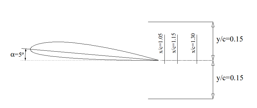
The data provided have been acquired at a distance of, approximately, \(\frac{x}{c} \approx 1.1\), where \(c = 265 \,\text{mm}\) is the profile’s chord. and there are 17 \(y\) positions, from \(y=-4 \,\text{cm}\) to \(y=+4 \,\text{cm}\), in intervals of 5 mm. In each point the velocity has been acquired for a second with a frequency of 1 kHz (that is, 1000 velocities in each point). It has been measured only the \(x\) component (main flow direction).

Most of the topics covered in this notebook have been consulted in the CFD-online Wiki page “Introduction to turbulence”

import pandas as pd
import numpy as np

We define the names for the columns, according with the definition

columns = []
for i in range(17):
    y = (i-8)*5
    columns.append("y = "+str(y)+"mm")

turbulenceData = pd.read_csv('TurbVel.csv',delimiter=',', index_col=0,names=columns)

turbulenceData.index.name="Time"

turbulenceData.head()

	y = -40mm	y = -35mm	y = -30mm	y = -25mm	y = -20mm	y = -15mm	y = -10mm	y = -5mm	y = 0mm	y = 5mm	y = 10mm	y = 15mm	y = 20mm	y = 25mm	y = 30mm	y = 35mm	y = 40mm
Time
0.000	20.916005	21.013892	19.890369	20.564816	19.247617	20.242762	20.171834	19.326923	17.711748	17.954515	19.112384	19.247617	18.955669	19.624038	18.989162	20.337691	17.901476
0.001	20.757920	21.124463	19.878740	20.528820	19.258909	20.278330	20.124676	19.417902	16.314876	17.534186	19.213710	19.292888	18.922264	19.704760	18.833365	20.313920	17.743229
0.002	20.661140	21.087559	20.101135	20.492846	19.213710	20.337691	20.136438	19.360977	13.902128	18.590930	19.202443	19.349631	18.933382	19.716296	18.601871	20.254624	17.922668
0.003	20.794288	21.099841	20.207287	20.421109	19.315560	20.219094	20.124676	19.349631	12.840679	18.340470	19.281544	19.372364	18.955669	19.785785	18.503472	20.278330	17.471901
0.004	20.952667	21.099841	20.349604	20.480892	19.292888	20.313920	20.148242	19.326923	15.086783	18.243283	19.247617	19.349631	18.944540	19.785785	17.838033	20.195451	18.135857

If we want to save this data in another file, keeping the information for index, columns, etc… instead of csv, we can use a more powerful format, as HDF. This is a Hierarchical Data Format, widely used to store big amounts of data in a organized way. More information, in the HDF group web page or in Wikipedia.

Warning

In ordert to save as HDF you will need the pytables module installed.

Just run

pip install tables

turbulenceData.to_hdf("TurbVel.hdf","w")

We can then get again the data with the format provided

newTurbulenceData = pd.read_hdf("TurbVel.hdf")

newTurbulenceData

	y = -40mm	y = -35mm	y = -30mm	y = -25mm	y = -20mm	y = -15mm	y = -10mm	y = -5mm	y = 0mm	y = 5mm	y = 10mm	y = 15mm	y = 20mm	y = 25mm	y = 30mm	y = 35mm	y = 40mm
Time
0.000	20.916005	21.013892	19.890369	20.564816	19.247617	20.242762	20.171834	19.326923	17.711748	17.954515	19.112384	19.247617	18.955669	19.624038	18.989162	20.337691	17.901476
0.001	20.757920	21.124463	19.878740	20.528820	19.258909	20.278330	20.124676	19.417902	16.314876	17.534186	19.213710	19.292888	18.922264	19.704760	18.833365	20.313920	17.743229
0.002	20.661140	21.087559	20.101135	20.492846	19.213710	20.337691	20.136438	19.360977	13.902128	18.590930	19.202443	19.349631	18.933382	19.716296	18.601871	20.254624	17.922668
0.003	20.794288	21.099841	20.207287	20.421109	19.315560	20.219094	20.124676	19.349631	12.840679	18.340470	19.281544	19.372364	18.955669	19.785785	18.503472	20.278330	17.471901
0.004	20.952667	21.099841	20.349604	20.480892	19.292888	20.313920	20.148242	19.326923	15.086783	18.243283	19.247617	19.349631	18.944540	19.785785	17.838033	20.195451	18.135857
...	...	...	...	...	...	...	...	...	...	...	...	...	...	...	...	...	...
0.995	21.087559	21.248015	19.349631	20.007225	19.785785	19.832212	19.612552	18.844470	17.010890	18.877784	17.234927	19.937022	20.373413	18.800155	17.451182	18.922264	19.808986
0.996	21.013892	21.334855	19.474945	19.972095	19.774176	19.855463	19.601036	18.844470	16.960352	18.082340	17.513403	20.183621	20.148242	18.800155	17.440815	19.532177	20.207287
0.997	21.050677	21.310005	19.440708	20.054129	19.704760	19.867080	19.578058	18.888878	16.373577	18.623839	17.680285	19.960385	20.148242	18.329634	17.461523	19.797365	20.160017
0.998	21.001619	21.297609	19.452103	20.054129	19.727874	19.832212	19.681671	18.933382	15.899636	18.039642	17.440815	19.693194	20.709496	18.211012	17.607118	19.601036	20.183621
0.999	21.062977	21.272798	19.497812	20.112884	19.612552	19.855463	19.658606	19.045057	16.570464	17.173579	17.327294	19.532177	20.721574	18.050324	17.378822	19.486393	20.065853

1000 rows × 17 columns

del(newTurbulenceData)

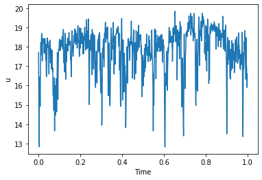
We can easily plot velocity time series in any point

turbulenceData["y = 0mm"].plot(ylabel="u")

<AxesSubplot:xlabel='Time', ylabel='u'>

And also we can get the main features

statData = turbulenceData.describe()
statData

	y = -40mm	y = -35mm	y = -30mm	y = -25mm	y = -20mm	y = -15mm	y = -10mm	y = -5mm	y = 0mm	y = 5mm	y = 10mm	y = 15mm	y = 20mm	y = 25mm	y = 30mm	y = 35mm	y = 40mm
count	1000.000000	1000.000000	1000.000000	1000.000000	1000.000000	1000.000000	1000.000000	1000.000000	1000.000000	1000.000000	1000.000000	1000.000000	1000.000000	1000.000000	1000.000000	1000.000000	1000.000000
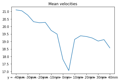
mean	21.104367	21.044473	20.757320	20.316435	20.247308	20.270573	19.733937	19.493431	17.798975	17.059820	19.138614	19.377307	19.330135	19.228752	19.026175	19.121565	18.570242
std	0.187226	0.228523	0.762061	0.776583	0.536762	0.262442	0.251107	0.491538	1.124547	0.988907	0.305786	0.354726	0.462051	0.478166	0.694788	0.662401	0.860208
min	20.468907	20.207287	18.634798	18.866662	19.123603	19.704760	19.168608	18.297226	12.824605	13.765816	17.234927	17.764286	17.245155	17.265657	16.373577	16.511184	16.101291
25%	20.989390	20.989390	20.322845	19.751012	19.797365	20.065853	19.566596	19.075895	17.327294	16.491465	18.977981	19.213710	19.109572	18.989162	18.678760	18.722815	17.983749
50%	21.099841	21.112168	20.733695	20.225018	20.272393	20.219094	19.704760	19.532177	18.071674	17.173579	19.168608	19.440708	19.338256	19.258909	19.045057	19.258909	18.689782
75%	21.173826	21.186155	21.062977	20.624988	20.676252	20.492846	19.913683	19.937022	18.569031	17.774791	19.315560	19.601036	19.658606	19.520739	19.477807	19.601036	19.227838
max	21.647802	21.447038	23.727658	23.157105	21.774209	20.842895	20.361487	20.661140	19.843817	19.727874	20.077620	20.230943	20.721574	20.444995	20.830752	20.337691	20.492846

statData.loc["mean"].plot(title="Mean velocities")

<AxesSubplot:title={'center':'Mean velocities'}>

2. Computation of turbulence intensities

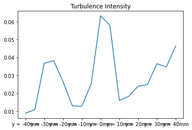
Remember the definition of turbulence intensity:

\[ I = \frac{\sqrt{\overline{u'^2}}}{\bar{u}} \tag{1} \]

where the numerator is, precisely, the std index of our statistical data.

turbIntensity = statData.loc["std"]/statData.loc["mean"]

turbIntensity.plot(title="Turbulence Intensity")

<AxesSubplot:title={'center':'Turbulence Intensity'}>

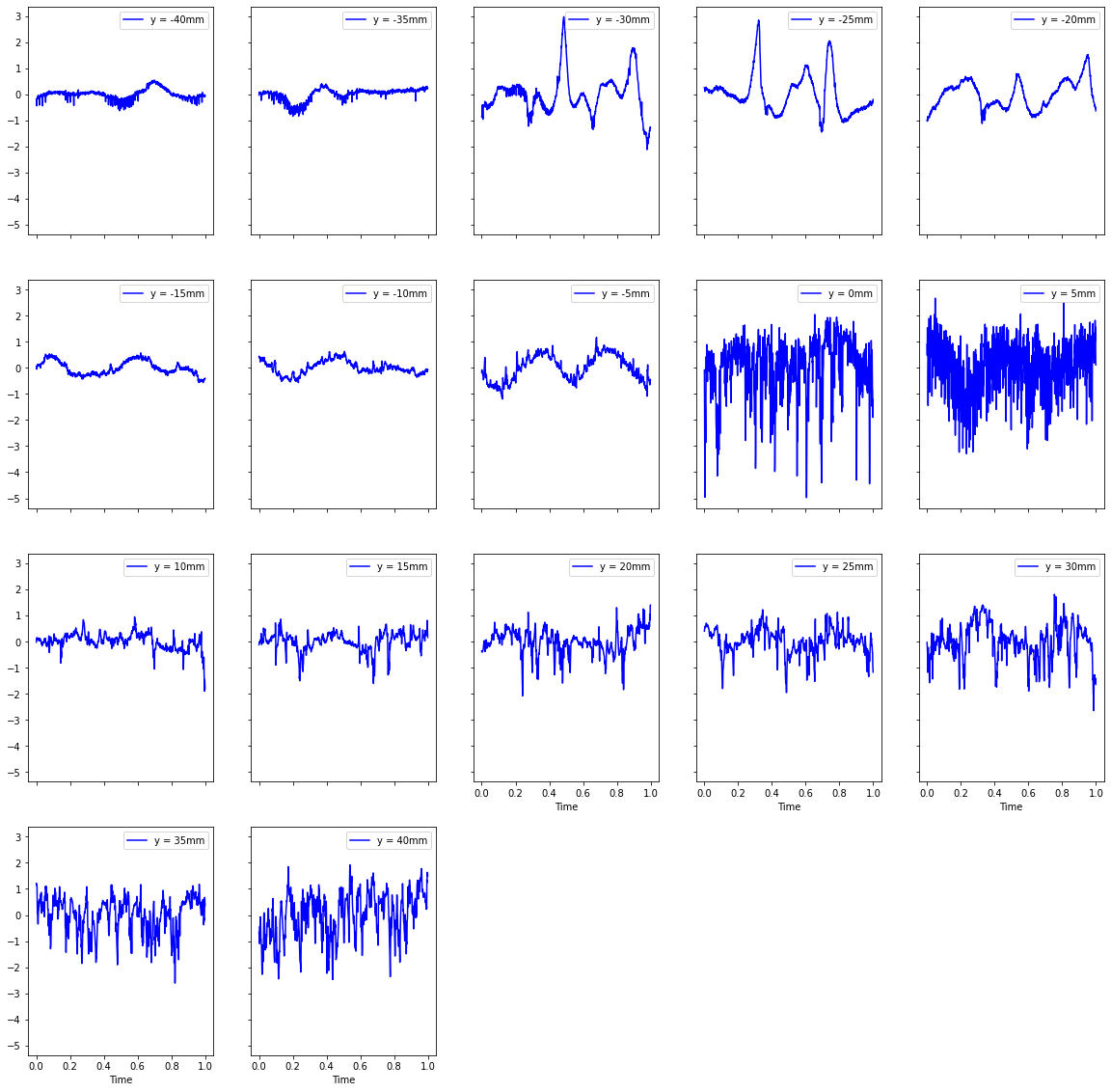
3. Computation of fluctuations

By definition, in each point the fluctuation of velocity is

\[ u' = u - \overline{u} \tag{2}\]

turbVelFluct = turbulenceData-statData.loc["mean"]

turbVelFluct.plot(subplots=True,layout=(4,5),figsize=(20,20),color="b",sharey=True);

4. Computation of turbulence kinetic energy

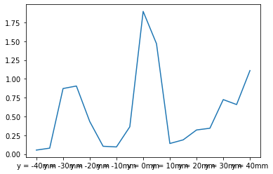
The turbulent kinetic energy (TKE), \(k\) is computed as

\[ k = \frac{1}{2}\overline{\boldsymbol{u'}\cdot\boldsymbol{u'}} = \frac{1}{2} \overline{u'_i u'_i} \tag{3}\]

and we should need also \(v'\) and \(w'\). We are then only computing the contribution of \(u'\) to TKE. Note that although main flow is in the \(x\) direction and components of velocities \(u\) and \(v\) can be neglected, it is not possible for fluctuating velocities \(v'\) and \(w'\). They can be as important as \(u'\). We can make the assumption that turbulence, at small scales, is isotropic and, hence \(\overline{u'}^2 \approx \overline{v'}^2 \approx \overline{w'}^2 \) and

\[ k \approx \frac{3}{2}\overline{u'}^2 \tag{4}\]

TKE = 1.5*statData.loc["std"]**2

TKE.plot()

<AxesSubplot:>

5. Some time scales

For the moment, we focus on \(y = 0 \,\text{mm}\) time series. The TKE in this point is

k = TKE.loc["y = 0mm"]
k

1.8969099438209802

The turbulence Reynolds number, locally defined in this point, is calculated with a length scale, which can be estimated, for now, as the larger eddy in the flow, of the order of the profile’s chord.

\[ \text{Re}_t = \frac{\sqrt{k}c}{\nu} \tag{5}\]

We need also the viscosity of air.

nu = 1.5e-5 # m^2/s
c = 0.265 # m
Re_t = np.sqrt(k)*c/nu
print('Re_t = {:.5g}'.format(Re_t))

Re_t = 24332

The Kolmogorov time scale can be estimated as

\[ \tau_k = \sqrt{\frac{\nu}{\varepsilon}} \tag{6}\]

where \(\varepsilon\) is the energy dissipation rate, that can be estimated as

\[ \varepsilon = \frac{k^{\frac{3}{2}}}{c} \tag{7}\]

(it is considered that energy is injected at larger scales)

epsilon = k**1.5/c
epsilon # m^2/s^3

9.858803164295557

And the Kolmogorov time scale is, approximately,

tau_k = np.sqrt(nu/epsilon)
tau_k

0.0012334840317132266

that is of the order of our time resolution.

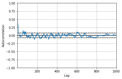
An integral time scale is defined with the autocorrelation of time signal.

\[ R(\tau) = \overline{u'(t)u'(t+\tau)} \tag{8}\]

Computing autocorrelation is very time consuming, but pandas has a plotting method that performs this computation much faster. The problem is that the output is directly a plot, and it is tricky to get the autocorrelation values from it.

uPrime = turbVelFluct["y = 0mm"].values
pd.plotting.autocorrelation_plot(uPrime);

autocorr = pd.plotting.autocorrelation_plot(uPrime).get_lines()[5].get_xydata()

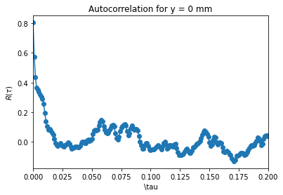
We change the “lag” \(x\) numbers with time lag, form the Data Frame

autocorr[:,0]=turbVelFluct.index.values

And also zoom for a narrower \(x\) span. Note that the pandas function gives the normalized correlation \(\rho(\tau)=\frac{R(\tau)}{R(0)} \).

import matplotlib.pyplot as plt
plt.plot(autocorr[:,0],autocorr[:,1],'o-')
ax = plt.gca()
ax.set_xlim(0,0.2)
ax.set_ylabel(r"$R(\tau)$")
ax.set_xlabel(r"\tau")
ax.set_title("Autocorrelation for y = 0 mm");

The integral time scale is defined as the integral of autocorrelation function

from scipy import integrate
T = integrate.trapezoid(autocorr[:,1],autocorr[:,0])
T

-0.0009022706750520157

It gives a very small (negative) value because the number of samples (1000) is still very low to get a good autocorrelation for large lag. It is assumed that after the second or third root, the autocorrelation is zero. So, we change the limits of integration:

T = integrate.trapezoid(autocorr[0:50,1],autocorr[0:50,0])
T

0.0038772428514055016

This method has the inconvenient that there is not the lag 0. It should be included in the very first point.

Alternatively, the statistic models package provides a better way to estimate autocorrelation, even with the option of choosing the number of lags for the computation.

import statsmodels.api as sm
rho = sm.tsa.acf(uPrime,nlags=50,fft=False)
rho

array([ 1.00000000e+00,  8.04541350e-01,  5.73932067e-01,  4.34197820e-01,
        3.66033657e-01,  3.52249759e-01,  3.37537587e-01,  3.17333281e-01,
        3.02811025e-01,  2.88497039e-01,  2.57130409e-01,  1.92849680e-01,
        1.36546784e-01,  1.03957571e-01,  8.32353264e-02,  8.38373665e-02,
        7.86032962e-02,  6.10277646e-02,  4.65580669e-02,  1.99746693e-02,
       -9.26964982e-03, -2.42545223e-02, -2.72775430e-02, -1.88646766e-02,
       -9.32923832e-03, -1.87112884e-02, -2.96367351e-02, -3.06195932e-02,
       -2.30782249e-02, -1.88316863e-02, -1.35537818e-02, -3.97915265e-03,
       -1.47696686e-02, -3.43907404e-02, -4.63080674e-02, -4.27395164e-02,
       -3.48795246e-02, -3.31582168e-02, -3.40160661e-02, -3.72166240e-02,
       -3.81736376e-02, -2.71323604e-02, -7.79263410e-03,  2.27309238e-03,
        5.12746823e-04, -1.00859193e-02, -1.05058317e-02,  9.75072762e-03,
        1.29933159e-02,  7.25182676e-03,  8.90439779e-03])

import statsmodels.graphics.api as smg
smg.tsa.plot_acf(uPrime,lags=200,fft=False)

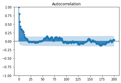
The computation of the integral time is more accurate because of the 0-lag point.

T = integrate.trapezoid(rho[0:50],autocorr[0:50,0])
T

0.004771435414182847

6. Histogram and PDF

PDF is the Probability Density Function. It defines the probability of an event between to values. For example, if the pdf of our velocity fluctuation is \(f(x)\), then the probability that a value of the fluctuation lies between \(u'_1\) and \(u'_2\) is

\[ P\left(u'_1 < u' < u'_2\right) = \int_{u'_1}^{u'_2} f(x) \text{d}x \tag{9}\]

import scipy.stats as stats
X = stats.norm(0,statData["y = 0mm"].loc["std"])
X_samples= X.rvs(1000)
F, bins, patches = plt.hist(uPrime,bins=100,density=True) # Integral = 1
plt.hist(X_samples,bins=100,density=True);

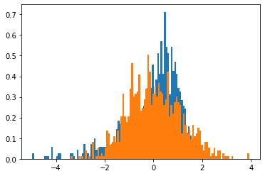
Since we have included the option density=True, the integral (moment of order 0) of this PDF is 1.

\[ M_0 = \int_{-\infty}^{+\infty} f(u') \text{d}u' = 1 \tag{10}\]

deltaUPrime = np.diff(bins) 
M0 = np.sum(F*deltaUPrime)
M0

1.0

The moment of order \(n\) is defined as

\[ M_n = \int_{-\infty}^{+\infty} u'^n f(u') \text{d}u' \tag{11}\]

The moment of order 1 is the average of the samples, that should be 0

\[ M_1 = \overline{u'} = \int_{-\infty}^{+\infty} u' f(u') \text{d}u' = 0 \tag{12}\]

UPrimePDF = bins[:-1] + deltaUPrime/2
UPrimePDF
M1 = np.sum(UPrimePDF*F*deltaUPrime)
M1

-0.00034572943202194895

The moment of order 2 is the variance of the samples, that should be the square of the standard deviation given by pandas before…

\[ M_2 = \overline{u'^2} = \int_{-\infty}^{+\infty} u'^2 f(u') \text{d}u' \tag{13}\]

M2 = np.sum(UPrimePDF**2*F*deltaUPrime)
M2

1.2646119129824565

We can check it easily with the statistical data

statData["y = 0mm"].loc["std"]**2

1.2646066292139868

The moment of order 3 is

\[ M_3 = \overline{u'^3} = \int_{-\infty}^{+\infty} u'^3 f(u') \text{d}u' \tag{14}\]

The skewness of the \(u'\) distribution is defined as

\[ S = \frac{M_3}{M_2^\frac{3}{2}} \tag{15}\]

M3 = np.sum(UPrimePDF**3*F*deltaUPrime)
M3

-1.9216881739274576

S = M3/M2**1.5
S

-1.351285182374243

The moment of order 4 is

\[ M_4= \overline{u'^4} = \int_{-\infty}^{+\infty} u'^4 f(u') \text{d}u' \tag{16}\]

The kurtosis of the \(u'\) distribution is defined as

\[ K = \frac{M_4}{M_2^2} \tag{17}\]

For a normal distribution, it should be 3 (check it)

M4 = np.sum(UPrimePDF**4*F*deltaUPrime)
M4

8.337551070336596

K = M4/M2**2
K

5.21343507900745

7. Power spectrum

Finally, from the time series signal, we can get the spectrum in frequency by performing a Fast Fourier Transform

E = np.abs(np.fft.fft(uPrime))
plt.plot(E);

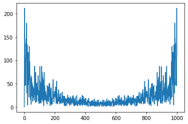
We compute the frequencies range, providing the periode of the data acquisition

freq = np.fft.fftfreq(uPrime.size,0.001)
plt.plot(freq,E);

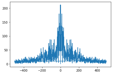
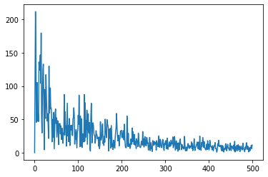
and we keep only half the data, since it is symmetric

E = E[:len(E)//2]
freq = freq[:len(freq)//2]
plt.plot(freq,E);

and, finally, we compute the energy, which is the square of the velocity

P = E**2
plt.plot(freq,E)

[<matplotlib.lines.Line2D at 0x7f1742ac86a0>]

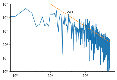
Let’s plot it in a log-log graph with the -5/3 Kolmogorov’s law as a reference line for the energy decay in frequency

fig, ax = plt.subplots(1)
ax.set_ylim(1,1e5)
ax.loglog(freq,P)
f_plot = np.logspace(1,2.7,100)
f_ref = 10 #Just a Frequancy and Energy of reference for the -5/3 law
P_ref = 1e5
P_plot = P_ref/f_ref**(-5/3)*f_plot**(-5/3)
ax.loglog(f_plot,P_plot,'--')
ax.text(30,20000,'-5/3');

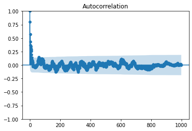
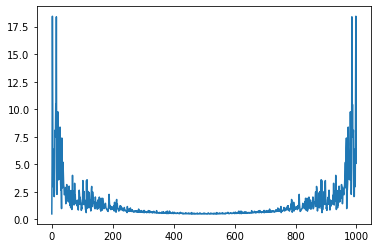
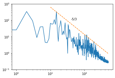
This spectrum can also be computed via the velocity autocorrelation

rho = sm.tsa.acf(uPrime,nlags=999,fft=False)
smg.tsa.plot_acf(uPrime,lags=999,fft=False)

Pr = np.abs(np.fft.fft(rho))
plt.plot(Pr);

freq = np.fft.fftfreq(rho.size,0.001)
Pr = Pr[:int(len(Pr)/2)]**2
freq = freq[:int(len(freq)/2)]

fig, ax = plt.subplots(1)
ax.set_ylim(0.1,1000)
ax.loglog(freq,Pr)
f_plot = np.logspace(1,2.7,100)
f_ref = 30
P_ref = 100
P_plot = P_ref/f_ref**(-5/3)*f_plot**(-5/3)
ax.loglog(f_plot,P_plot,'--')
ax.text(40,100,'-5/3');

try:
    %load_ext watermark
except:
    !pip install watermark
%watermark -v -m -iv

Python implementation: CPython
Python version       : 3.8.13
IPython version      : 8.0.1

Compiler    : GCC 10.3.0
OS          : Linux
Release     : 5.4.0-144-generic
Machine     : x86_64
Processor   : x86_64
CPU cores   : 4
Architecture: 64bit

matplotlib : 3.5.1
statsmodels: 0.13.2
pandas     : 1.4.2
numpy      : 1.22.2
scipy      : 1.8.1