Introduction to scientific computation with Python#
Python is a high level computational language. It is quite similar to Matlab, but with the advantage that is is open source, free and internet is plenty of libraries that allow to solve a large variety of problems.
The main libraries used in scientific computations are numpy for numerical computation, sympy for Computer Albegra System (CAS), matplotlib for plotting, and pandas for data analysis. All this packages are collected in the scipy ecosystem.
One practical way to compute with python is a Jupyter notebook, like the present one. It allows to combine text, equations, graphs and pictures with code. One of the most interesting features of a Jupyter Notebook is that it is interactive. That means that the user can download, open and play with it.
All that can be installed in any system (Windows, Mac, Linux,…) (and even in an android phone!) but it is highly recommended to install through an special distribution. The most popular is now Anaconda that has free and paid versions. However, recently it has been launched an small multi-platform application called Jupyterlab Desktop that is very recommended because of its size and practicality.
1. Numpy#
Python is a powerful language. Its power lies mainly in its modulability. With naked python few interesting things can be done. But modules of libraries can be easily imported and used to perform almost everything we need.
In maths and science, one of the main modules is numpy, which gives acces to numerical computations with arrays, matrix, functions, … with optimized performance.
To import a module in python is very easy (as long as it is installed in the system…). Just type
import numpy
and access any component of the library with, por example
numpy.log(3)
1.0986122886681098
Another way to import a module is with
from numpy import *
and then you can use the same components without need of type the word numpy everytime
log(3)
1.0986122886681098
The last way is with
import numpy as np
np.log(3)

This last is my favorite, but you can use whichever you prefer.
If the module is not installed in the system it can be easily downloaded and installed with a pip (Package Installer for Python) command in a python cell:
!pip install numpy
The ! symbols is to scape to shell to execute the command.
To get fast information about any component of python or any module, just type a ‘?’ at the end of the command
np.log?
Call signature:  np.log(*args, **kwargs)
Type:            ufunc
String form:     <ufunc 'log'>
File:            ~/.config/jupyterlab-desktop/jlab_server/lib/python3.8/site-packages/numpy/__init__.py
Docstring:
log(x, /, out=None, *, where=True, casting='same_kind', order='K', dtype=None, subok=True[, signature, extobj])

Natural logarithm, element-wise.

The natural logarithm `log` is the inverse of the exponential function,
so that `log(exp(x)) = x`. The natural logarithm is logarithm in base
`e`.

Parameters
----------
x : array_like
    Input value.
out : ndarray, None, or tuple of ndarray and None, optional
    A location into which the result is stored. If provided, it must have
    a shape that the inputs broadcast to. If not provided or None,
    a freshly-allocated array is returned. A tuple (possible only as a
    keyword argument) must have length equal to the number of outputs.
where : array_like, optional
    This condition is broadcast over the input. At locations where the
    condition is True, the `out` array will be set to the ufunc result.
    Elsewhere, the `out` array will retain its original value.
    Note that if an uninitialized `out` array is created via the default
    ``out=None``, locations within it where the condition is False will
    remain uninitialized.
**kwargs
    For other keyword-only arguments, see the
    :ref:`ufunc docs <ufuncs.kwargs>`.

Returns
-------
y : ndarray
    The natural logarithm of `x`, element-wise.
    This is a scalar if `x` is a scalar.

See Also
--------
log10, log2, log1p, emath.log

Notes
-----
Logarithm is a multivalued function: for each `x` there is an infinite
number of `z` such that `exp(z) = x`. The convention is to return the
`z` whose imaginary part lies in `[-pi, pi]`.

For real-valued input data types, `log` always returns real output. For
each value that cannot be expressed as a real number or infinity, it
yields ``nan`` and sets the `invalid` floating point error flag.

For complex-valued input, `log` is a complex analytical function that
has a branch cut `[-inf, 0]` and is continuous from above on it. `log`
handles the floating-point negative zero as an infinitesimal negative
number, conforming to the C99 standard.

References
----------
.. [1] M. Abramowitz and I.A. Stegun, "Handbook of Mathematical Functions",
       10th printing, 1964, pp. 67.
       https://personal.math.ubc.ca/~cbm/aands/page_67.htm
.. [2] Wikipedia, "Logarithm". https://en.wikipedia.org/wiki/Logarithm

Examples
--------
>>> np.log([1, np.e, np.e**2, 0])
array([  0.,   1.,   2., -Inf])
Class docstring:
Functions that operate element by element on whole arrays.

To see the documentation for a specific ufunc, use `info`.  For
example, ``np.info(np.sin)``.  Because ufuncs are written in C
(for speed) and linked into Python with NumPy's ufunc facility,
Python's help() function finds this page whenever help() is called
on a ufunc.

A detailed explanation of ufuncs can be found in the docs for :ref:`ufuncs`.

**Calling ufuncs:** ``op(*x[, out], where=True, **kwargs)``

Apply `op` to the arguments `*x` elementwise, broadcasting the arguments.

The broadcasting rules are:

* Dimensions of length 1 may be prepended to either array.
* Arrays may be repeated along dimensions of length 1.

Parameters
----------
*x : array_like
    Input arrays.
out : ndarray, None, or tuple of ndarray and None, optional
    Alternate array object(s) in which to put the result; if provided, it
    must have a shape that the inputs broadcast to. A tuple of arrays
    (possible only as a keyword argument) must have length equal to the
    number of outputs; use None for uninitialized outputs to be
    allocated by the ufunc.
where : array_like, optional
    This condition is broadcast over the input. At locations where the
    condition is True, the `out` array will be set to the ufunc result.
    Elsewhere, the `out` array will retain its original value.
    Note that if an uninitialized `out` array is created via the default
    ``out=None``, locations within it where the condition is False will
    remain uninitialized.
**kwargs
    For other keyword-only arguments, see the :ref:`ufunc docs <ufuncs.kwargs>`.

Returns
-------
r : ndarray or tuple of ndarray
    `r` will have the shape that the arrays in `x` broadcast to; if `out` is
    provided, it will be returned. If not, `r` will be allocated and
    may contain uninitialized values. If the function has more than one
    output, then the result will be a tuple of arrays.
2. Sympy#
With the library sympy symbolic manipulation of mathematical equations can be performed, in a similar way as with Maple, Mathematica or Wolfram Alpha.
The command
try:
    ...
except:
    ...
tries to execute something (in this case, it tries to import sympy) and, if it fails, run the command in except:, in this case, it install
the version 1.7.1 of sympy.
try:
    import sympy as sp
except:
    !pip install sympy==1.7.1
The first step to perform symbolic computation is to declare the symbols that are going to used
x,y = sp.symbols('x,y')
If, in addition, we include the command
sp.init_printing()
the ouput will be nicely rendered in a Jupyter notebook
sp.sqrt(x)

An expression can be build with our symbols
expr = 1+2*x**2*(x-1)-x**3
display(expr)

and it can be simplified, either with
sp.simplify(expr)

or with
expr.simplify()

Expressions can be factorized
expr = expr.factor()
display(expr)

or expanded again
expr = expr.expand()
display(expr)

We can solve equations, by defining an equality of two expressions with the sympy.Eq() class
equation = sp.Eq(y,expr)
display(equation)

x_sol = sp.solve(equation,x)
display(x_sol)

It gives 3 complex solutions. We can access to each of them as member of an array
display(x_sol[0])

Or we can solve systems of equations
eq1 = x + 2*y - 1
display(eq1)
eq2 = x - y + 1
display(eq2)
eq_sol = sp.solve([eq1,eq2],[x,y])
display(eq_sol)


We can make substitutions in an expression, with subs()
expr = expr.subs(x,x+1)
display(expr)

or with replace() that is often more powerful
expr = expr.replace(x,3*x)
display(expr)

Several substitutions can be performed by means of a dictionary
changes = {y:sp.cos(y),x:sp.sqrt(x)}
equation = equation.subs(changes)
display(equation)

We can also perform numerical evaluations.
The best way is with a lambda method that creates a function to evaluate any value
expr_func = sp.lambdify(x,expr)
expr_func(2.0)

Manipulating algebraic functions and solvind ODEs#
Besides symbols, we can define functions, and its derivatives
f = sp.Function('f')
display(f(x))
display(f(x).diff(x))
display(f(x).diff(x,2))


In this case, the function \(f(x)\) is not defined and sympy can just represents symbolicaly its derivative. But we can
make the derivative of any expression
expr.diff(x)

expr.diff(x,2)

Also we can, of course, integrate a function
f(x).integrate()

f(x).integrate((x,0,sp.pi))

expr.integrate()

expr.integrate((x,0,1))

We can calculate series expansion, both symbolicaly
f(x).series(x)

f(x).series(x,1)

f(x).series(x,1,n=2)

f(x).series(x,1,n=2).removeO()

or explicitely
sqrt_x = sp.sqrt(x)
display(sqrt_x)

sqrt_x.series(x,1,n=3)

sqrt_x.series(x,1,n=3).removeO()

Let’s now solve an ODE
Let’s consider the first order ODE for Newton’s cooling law
with \(T(0) = T_0\).
t,k,Ta,T0 = sp.symbols('t,k,T_a,T_0')
T = sp.Function("T")
ode = sp.Eq(T(t).diff(t),-k*(T(t)-Ta))
display(ode)

ode_sol = sp.dsolve(ode)
display(ode_sol)

and it can be done directly with the initial condition
ode_sol = sp.dsolve(ode,ics={T(0):T0})
display(ode_sol)

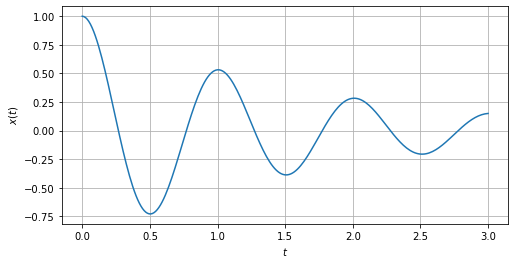
For a second order ODE, let’s consider a damped harmonic oscillator
t,omega0,gamma = sp.symbols('t,omega0,gamma',positive=True)
x = sp.Function('x')
ode2 = sp.Eq(x(t).diff(t,2)+2*gamma*omega0*x(t).diff(t)+omega0**2*x(t),0)
display(ode2)

ode2_sol = sp.dsolve(ode2)
display(ode2_sol)

The boundary conditions are that \(x=1\) and its derivative is 0 for \(t=0\).
ics = {x(0):1,x(t).diff(t).subs(t,0):0}
ode2_sol = sp.dsolve(ode2,ics=ics)
display(ode2_sol)

We see now how to plot a particular case of this equations by using matplotlib
we are going to consider the case \(\omega_0 = 2\pi\) and \(\gamma = 0.1\)
import matplotlib.pyplot as plt
%matplotlib inline
values = {omega0: 2*sp.pi,gamma:0.1}
fig,ax = plt.subplots(figsize=(8,4))
tt = np.linspace(0,3,250)
x_t = sp.lambdify(t,ode2_sol.rhs.subs(values))
ax.plot(tt,x_t(tt).real) # There are some complex results. We take only the real part
ax.set_xlabel(r'$t$')
ax.set_ylabel(r'$x(t)$')
ax.grid(which='major',axis='both')
Example: Solving the equation of motion of a roquet#
In this example we are going to use sympy to solve the equation of motion of a roquet, as described in many basic Fluid Mechanics textbook. See, for instance, example 3.12 of White’s book
import sympy as sp
m0,mDot,t,vg = sp.symbols('m_0,\dot{m},t,v_g')
v = sp.Function('v')
ode = sp.Eq((m0+mDot*t)*v(t).diff(t),-mDot*vg)
display(ode)

condCont = {v(0):0}
sol = sp.dsolve(ode,ics=condCont)
display(sol)

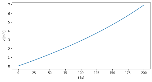
We test and plot the solutions with some random values:
values = {mDot:-1,m0:400,vg:10}
v_t = sp.lambdify(t,sol.rhs.subs(values))
import matplotlib.pyplot as plt
import numpy as np
tt = np.linspace(0,200,250)
vtt = v_t(tt)
fig,ax = plt.subplots(figsize=(8,4))
ax.plot(tt,vtt)
ax.set_xlabel(r'$t$ [s]')
ax.set_ylabel(r'$v$ [m/s]');
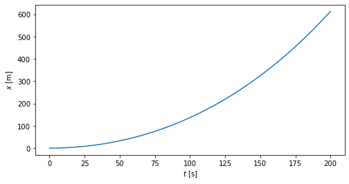
x = sol.rhs.integrate((t,0,t))
display(x)

x_t = sp.lambdify(t,x.subs(values))
xtt = x_t(tt)
fig,ax = plt.subplots(figsize=(8,4))
ax.plot(tt,xtt)
ax.set_xlabel(r'$t$ [s]')
ax.set_ylabel(r'$x$ [m]');
3. Pandas#
Pandas is a library for data analysis. Is some kind of powerful datasheet. Documentation is here.
The two main data structures are Series and DataFrame
Series#
A Series is an array that can be indexed with labels instead of integers
For example, we can make a Series with grades in some subjects
import pandas as pd
grades = pd.Series([5.5,7.6,4.3,8.6,6.5])
grades
0    5.5
1    7.6
2    4.3
3    8.6
4    6.5
dtype: float64
grades.index
RangeIndex(start=0, stop=5, step=1)
This is the array inside the Series
grades.values
array([5.5, 7.6, 4.3, 8.6, 6.5])
And now we can changes index
grades.index = ["Maths","Spanish","Catalan","Physics","German"]
grades.name = "Grades"
grades
Maths      5.5
Spanish    7.6
Catalan    4.3
Physics    8.6
German     6.5
Name: Grades, dtype: float64
That could be also done with
It is easy to access to some values
grades["Physics"]

grades[["Maths","Physics","German"]]
Maths      5.5
Physics    8.6
German     6.5
Name: Grades, dtype: float64
Some statistics:
print("Median of grades is {0}".format(grades.median()))
print("Mean of grades is {0}".format(grades.mean()))
print("Standard deviation of grades is {0}".format(grades.std()))
print("Maximum of grades is {0}".format(grades.max()))
print("Minimum of grades is {0}".format(grades.min()))
print("Quartile of grades is {0}".format(grades.quantile(0.25)))
Median of grades is 6.5
Mean of grades is 6.5
Standard deviation of grades is 1.6926310879810755
Maximum of grades is 8.6
Minimum of grades is 4.3
Quartile of grades is 5.5
Also, in brief
grades.describe()
count    5.000000
mean     6.500000
std      1.692631
min      4.300000
25%      5.500000
50%      6.500000
75%      7.600000
max      8.600000
Name: Grades, dtype: float64
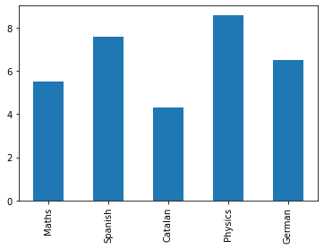
Plot method can be used for easily plot data
import matplotlib.pyplot as plt
fig,axes = plt.subplots()
grades.plot(kind='bar')
<AxesSubplot:>
DataFrame#
It is like a multidimensional Series. Typically, a table
subjects = pd.DataFrame(grades)
subjects.columns
Index(['Grades'], dtype='object')
subjects
| Grades | |
|---|---|
| Maths | 5.5 |
| Spanish | 7.6 |
| Catalan | 4.3 |
| Physics | 8.6 |
| German | 6.5 |
teachers = pd.Series(["Dave","Ana","John","Grace","Mike"],name="Teacher",index = ["Maths","Spanish","Catalan","Physics","German"])
subjects = subjects.join(teachers)
subjects
| Grades | Teacher | |
|---|---|---|
| Maths | 5.5 | Dave |
| Spanish | 7.6 | Ana |
| Catalan | 4.3 | John |
| Physics | 8.6 | Grace |
| German | 6.5 | Mike |
subjects.Grades.mean()

subjects.loc["Maths"]
Grades      5.5
Teacher    Dave
Name: Maths, dtype: object
subjects.Teacher
Maths       Dave
Spanish      Ana
Catalan     John
Physics    Grace
German      Mike
Name: Teacher, dtype: object
4. Data fitting#
Linear regression#
Some times we need to fit experimental data in order to create a model (a math expression). There are two main python modules to make it: statsmodels and patsy. Actually, statsmodel calls internally to patsy, and it is ususlly not necessary to explicitely import it, but we are doing it for the sake of clarity
#This command resets the python kernel, and remove all modules, variables and data
%reset -f
Note
If not done, you have to install the statsmodels module with
pip install statsmodel
try:
    import statsmodels.api as sm
except:
    !pip install statsmodel
import statsmodels.formula.api as smf
import statsmodels.graphics.api as smg
import patsy
import matplotlib.pyplot as plt
import numpy as np
import pandas as pd
Let’s consider the next image, taken from Wikipedia-Scatter Plot
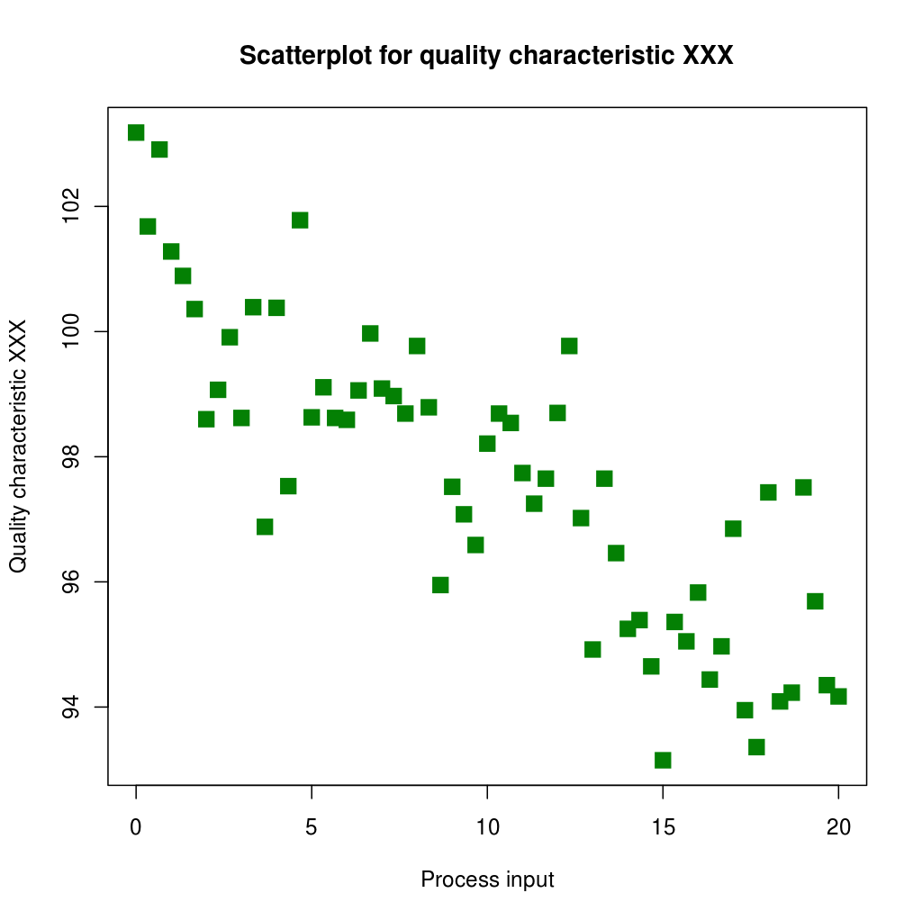
The first step is to get the data. It is done with a plot digitizer. There are several tools to do that: 3gdata for linux, the Java app Plot Digitizer or the online app Web Plot Digitizer. I recommend this last one. With this app we can generate a CSV file, that I have called “Scatter_data.csv”.
The second step is to load this data file into a pandas DataFrame
ScatterData = pd.read_csv("Scatter_data.csv",header=None,names=["x","y"]) # It's important the names for the columns data
ScatterData.head()
| x | y | |
|---|---|---|
| 0 | 0.011 | 103.186 |
| 1 | 0.344 | 101.689 |
| 2 | 0.678 | 102.855 |
| 3 | 1.011 | 101.286 |
| 4 | 1.344 | 100.897 |
We can plot it to check it…
plt.scatter(ScatterData["x"],ScatterData["y"])
<matplotlib.collections.PathCollection at 0x7fd454665fa0>
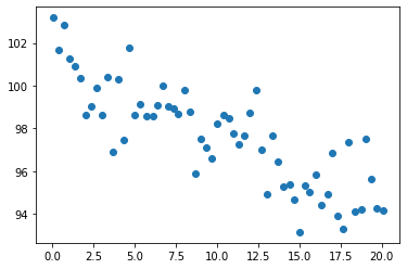
The third step is to create a model. We are using a formula for the model. Actually, it is just a linear regression, made with ordinary least square estimation. Check here how is the syntax for the formulae in patsy.
model = smf.ols("y~x",ScatterData)
That only creates the model, but does not compute anything. The computation is made with the fit method.
result = model.fit()
We check the result
result.summary()
| Dep. Variable: | y | R-squared: | 0.703 |
|---|---|---|---|
| Model: | OLS | Adj. R-squared: | 0.698 |
| Method: | Least Squares | F-statistic: | 139.8 |
| Date: | Sun, 05 Feb 2023 | Prob (F-statistic): | 3.34e-17 |
| Time: | 08:37:09 | Log-Likelihood: | -102.79 |
| No. Observations: | 61 | AIC: | 209.6 |
| Df Residuals: | 59 | BIC: | 213.8 |
| Df Model: | 1 | ||
| Covariance Type: | nonrobust |
| coef | std err | t | P>|t| | [0.025 | 0.975] | |
|---|---|---|---|---|---|---|
| Intercept | 101.0919 | 0.336 | 300.828 | 0.000 | 100.420 | 101.764 |
| x | -0.3422 | 0.029 | -11.824 | 0.000 | -0.400 | -0.284 |
| Omnibus: | 0.117 | Durbin-Watson: | 1.789 |
|---|---|---|---|
| Prob(Omnibus): | 0.943 | Jarque-Bera (JB): | 0.155 |
| Skew: | 0.095 | Prob(JB): | 0.925 |
| Kurtosis: | 2.841 | Cond. No. | 23.1 |
Notes:
[1] Standard Errors assume that the covariance matrix of the errors is correctly specified.
The result object has a lot of components. One is the params: the coefficient Intercept which is the independent term, and the x, which is, in this case, the kinear term coefficient.
display(result.params["Intercept"])
display(result.params["x"])


In the last step, let’s now plot it to see how it looks like.
First, we create the set of x points to make the plot. It has to be a pandas DataFrame.
x_plot = pd.DataFrame(pd.Series(np.linspace(0,20,250),name="x"))
and now we calculate the prediction, according to our linear model
y_plot = result.predict(x_plot)
x_plot
| x | |
|---|---|
| 0 | 0.000000 |
| 1 | 0.080321 |
| 2 | 0.160643 |
| 3 | 0.240964 |
| 4 | 0.321285 |
| ... | ... |
| 245 | 19.678715 |
| 246 | 19.759036 |
| 247 | 19.839357 |
| 248 | 19.919679 |
| 249 | 20.000000 |
250 rows × 1 columns
and, finally, we plot it
a = result.params["Intercept"]
b = result.params["x"]
plt.scatter(ScatterData["x"],ScatterData["y"])
plt.plot(x_plot.values,y_plot,"r-",linewidth=3)
plt.text(9.0,101,r"$y = {:.2f} {:+.2f}x$".format(a,b),color="red")
Text(9.0, 101, '$y = 101.09 -0.34x$')
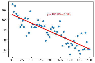
If we want to make another fit, for example, with a quadratic expression, we have to create another column in the DataFrame with the new data (in this case, with \(x^2\)). This is still considered a linear regression, since it can be written as linear combination of polynomical terms \( y = \sum_{n=0}^{N} a_n x^n\). Note also that a model as \(y=a_0x^{a_1}\), or \(y=a_0\exp(a_1x)\), can be tranformed into a linear model just calculating logarithm of both sides.
ScatterData["x2"] = ScatterData["x"]**2
ScatterData.head(3)
| x | y | x2 | |
|---|---|---|---|
| 0 | 0.011 | 103.186 | 0.000121 |
| 1 | 0.344 | 101.689 | 0.118336 |
| 2 | 0.678 | 102.855 | 0.459684 |
and then we create the new model, and perform the fit() method
sqr_model = smf.ols('y~ x + x2',ScatterData)
sqr_result = sqr_model.fit()
sqr_result.summary()
| Dep. Variable: | y | R-squared: | 0.706 |
|---|---|---|---|
| Model: | OLS | Adj. R-squared: | 0.696 |
| Method: | Least Squares | F-statistic: | 69.69 |
| Date: | Sun, 05 Feb 2023 | Prob (F-statistic): | 3.76e-16 |
| Time: | 08:37:29 | Log-Likelihood: | -102.49 |
| No. Observations: | 61 | AIC: | 211.0 |
| Df Residuals: | 58 | BIC: | 217.3 |
| Df Model: | 2 | ||
| Covariance Type: | nonrobust |
| coef | std err | t | P>|t| | [0.025 | 0.975] | |
|---|---|---|---|---|---|---|
| Intercept | 101.3684 | 0.496 | 204.170 | 0.000 | 100.375 | 102.362 |
| x | -0.4262 | 0.114 | -3.724 | 0.000 | -0.655 | -0.197 |
| x2 | 0.0042 | 0.006 | 0.759 | 0.451 | -0.007 | 0.015 |
| Omnibus: | 0.048 | Durbin-Watson: | 1.807 |
|---|---|---|---|
| Prob(Omnibus): | 0.976 | Jarque-Bera (JB): | 0.166 |
| Skew: | 0.061 | Prob(JB): | 0.920 |
| Kurtosis: | 2.775 | Cond. No. | 540. |
Notes:
[1] Standard Errors assume that the covariance matrix of the errors is correctly specified.
sqr_result.params
Intercept    101.368371
x             -0.426238
x2             0.004192
dtype: float64
x2_plot = x_plot.join(pd.Series(x_plot["x"]**2,name="x2"))
x2_plot
| x | x2 | |
|---|---|---|
| 0 | 0.000000 | 0.000000 |
| 1 | 0.080321 | 0.006452 |
| 2 | 0.160643 | 0.025806 |
| 3 | 0.240964 | 0.058064 |
| 4 | 0.321285 | 0.103224 |
| ... | ... | ... |
| 245 | 19.678715 | 387.251819 |
| 246 | 19.759036 | 390.419509 |
| 247 | 19.839357 | 393.600103 |
| 248 | 19.919679 | 396.793600 |
| 249 | 20.000000 | 400.000000 |
250 rows × 2 columns
y2_plot = sqr_result.predict(x2_plot)
a = result.params["Intercept"]
b = result.params["x"]
a0 = sqr_result.params["Intercept"]
a1 = sqr_result.params["x"]
a2 = sqr_result.params["x2"]
fig,ax = plt.subplots()
ax.set_xlabel(r'$x$')
ax.set_ylabel(r'$y$')
ax.scatter(ScatterData["x"],ScatterData["y"])
ax.plot(x_plot.values,y_plot,"r-",linewidth=3)
ax.plot(x_plot.values,y2_plot,"g-",linewidth=3)
ax.text(9.0,101,r"$y = {:.2f} {:+.2g}x$".format(a,b),color="red")
ax.text(9.0,100,r"$y = {:.2f} {:+.2g}x {:+.2g}x^2$".format(a0,a1,a2),color="green")
Text(9.0, 100, '$y = 101.37 -0.43x +0.0042x^2$')
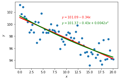
Non linear regression#
When we want to make a non linear regression, for instance to fit with a model as \(y=a_0+a_1*\exp{a_2*x}\), an optimization method to compute mininum squares has to be performed. We use then the optimize module of scipy, and, in particular, the curve_fit method.
import scipy.optimize as opt
import numpy as np
import matplotlib.pyplot as plt
We load the data. Now it can be just with an array instead of a pandas DataFrame.
[xdata,ydata] = np.loadtxt("Scatter_data.csv",delimiter=',').T #The traspose has to be made in order to load columns instead of rows
fig,ac = plt.subplots()
ac.scatter(xdata,ydata)
<matplotlib.collections.PathCollection at 0x7fd464c6e550>

We define the fitting function (our model) with the independent variable \(x\), and the set of parameters (the parameters name is free)
def f(x,a0,a1,a2):
    return a0+a1*np.exp(a2*x)
And we perform the curve fitting. Note the p0 argument. It gives an initial guess. Otherwise the iterative process can be very long and eventually, it an fail. It gives two results. The first is the solution. The second is the covariance matrix. The diagonal of this matrix is the statistical variance of the solutions.
popt, pcov = opt.curve_fit(f,xdata,ydata, p0=[100,1,-1])
[a0,a1,a2] = popt
Let’s calculate the predicted values of a uniform \(x\) distribution
xdata_plot = np.linspace(0,20,250)
ydata_plot = f(xdata_plot,a0,a1,a2)
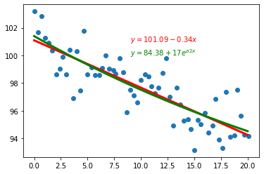
And let’s plot it, with comparison with linear regression.
fig,ax = plt.subplots()
ax.scatter(xdata,ydata)
ax.plot(x_plot.values,y_plot,"r-",linewidth=3)
ax.plot(xdata_plot,ydata_plot,"g-",linewidth=3)
ax.text(9.0,101,r"$y = {:.2f} {:+.2g}x$".format(a,b),color="red")
ax.text(9.0,100,r"$y = {:.2f} {:+.2g}e^{{a2 x}}$".format(a0,a1,a2),color="green")
Text(9.0, 100, '$y = 84.38 +17e^{a2 x}$')
The statsmodel ols gives the R-squared as part of the results.
result.rsquared

The scipy optimize doesn’t do this computation, but it is easy to perform by hand, as stated in this stackoverflow answer, according to wikipedia page.
residuals = ydata - f(xdata,a0,a1,a2)
ss_res = np.sum(residuals**2)
ss_tot = np.sum((ydata-np.mean(ydata))**2)
r_squared = 1 - (ss_res / ss_tot)
r_squared

In the next command, the watermark extension is used in order to register the version of the libraries used in the Notebook. This is useful for the reproductibility.
try:
    %load_ext watermark
except:
    !pip install watermark
%watermark -v -m -iv
Python implementation: CPython
Python version       : 3.8.13
IPython version      : 8.2.0

Compiler    : GCC 10.3.0
OS          : Linux
Release     : 5.4.0-137-generic
Machine     : x86_64
Processor   : x86_64
CPU cores   : 8
Architecture: 64bit

scipy      : 1.8.0
numpy      : 1.22.3
matplotlib : 3.5.1
patsy      : 0.5.2
statsmodels: 0.13.2
pandas     : 1.4.2


